Editing Your Tilia Data File

We are going to walk through the process of generating a Tilia record for your dataset in a way that is (at least to us) intuitive. This is not neccessarily the way that Tilia is set up by default. At any time you can navigate to a particular section through the sidebar. This set of instructions assumed that you have started a new file and loaded the appropriate lookup tables.

Overview of data entry process

Data entry through Tilia is an iterative process. For most datasets, it is easiest to start with the Data tab to enter the primary data (taxon names and counts at different depths/analysis units), then fill in the associated Metadata, then return to the Data tab to add contextual information. For some types of data, it is helpful to enter Specimen-level data early in the process, because they can then be easily linked to associated data such as radiocarbon dates (in the Geochronology tab) and Isotopes.

Data Tab

Entering New Data

Adding information on the depths/analysis units

Starting from a blank Data tab we can fill in some basic information about the individual analysis units from which you have counted or identified material. In some cases, Analysis Units are stored solely as depths, and in other cases they are stored solely by Analysis Unit names (i.e., many vertebrate data have names such as “Stratum 1” or “Level 10” or “East unit”). Both types of data can be entered as well. If your data has depths then these should be entered along the very top row (Row 1), starting with Column H. If your data has Analysis Unit names, these can be entered in Row 2, starting with Column H.

Quite a bit of additional information that describes the Analysis Units can be added if desired. This information is typically entered starting in Row 3. The process for entering these data is described below in “Annotating the Data”

Adding taxa

Taxon names should be entered in the ‘Name’ column (column B). If the appropriate lookup files have been loaded, starting to type will pull out a list of taxa and show you which taxonomic names match your entry. If the taxon is already in the database, selecting that taxon will autofill the Code (Column A) and Group (Column G) columns.

Then fill in the appropriate information for Columns C-F. + Double click cell and it should turn white with a down arrow on the right + Clicking the arrow should show a drop down menu from which to choose the appropriate information. + The most important information to add here is information on the Element and Units.

Adding data values

Once the backbone of the spreadsheet is started, values (counts, presence/absence, etc) can be entered. Note that the values will be interpreted in the context of the taxon, element, and units. Thus, you could have two rows associated with the same taxon, and one row is associated with the NISP value for that taxon at each Analysis Unit and the other row is associated with the MNI value for that taxon at each Analysis Unit.

Copying data from an Existing Spreadsheet

Note that data can be copied and pasted from a local spreadsheet (ie, excel or csv files) into the Data tab. Thus, if you have a list of taxonomic names, or a full spreadsheet of data arranged in the same format as the Tilia Data tab, you should be able to paste in the full dataset.

First, make sure the Depths or Analysis Unit names have been added. If depths are available, add them (midpoints, generally) to the first row, above the relevant named analysis unit.

If known, you can add the analyst too (e.g., if different people identified different strata within the deposit). To do this, add another row below thickness using the same procedure as above, adding Metadata → Sample Analyst. Then, go to the cell below the first analysis unit, regular click in the cell, and add the relevant contacts from the Contacts Tab. Once you’ve added the first cell, you can then copy and paste to other analysis units.

Next fill in the taxa list, starting directly below the header metadata. First fill out the Name column using the automatic pull down menu to select the taxon. This will automatically fill out the Code column and the Group column for you.

Element

the type of element representing that taxon. Typical faunal elements are bones, teeth, scales, and other hard body parts. Bone and tooth elements may be specifically identified (e.g. «tibia» or even more precisely «tibia, distal, left», «M2, lower, left»). Use the pull down menu.

Units

choose the appropriate unit that the data represent. If you have more than one unit type (e.g. Present/Absent, MNI and NISP), add a second row for that taxon and include data for the second unit type.

Context

add if known

Taphonomy

add if known

Data

Fill in the appropriate values for each cell, e.g., 1s or 0s if entering presence/absence data, or integer values if entering NISP or MNI

Adding Specimen Data

Once the assemblage data have been entered, you can then add any desired information on individual specimens. Specimen data can be associated with any value for Units.

To add specimens: + Click once on the cell where you want to add specimen information so that the cell has a black outline on it + Right click and select the “Specimens” option + This will open up a new popup on your screen where you will fill out the specimen data

Within the Specimens popup, some information will have associated structured values available through a drop-down menu and others will require manual entry. You can double click each to find out if there is a drop down menu or if you have to manually input your information. For example, “Element” cells have a drop down list of options, while “SpecID” is manually filled in.

Some cells cannot be filled in unless data has been entered into another cell first. The basic information needed is Spec ID. This is the analyst ID, however you wish to define it. This is the name that will appear in other tabs of the file (such as Geochronology or Isotopes). Any formal Specimen ID information can be added through Spec Nr and is expected to be associated with the selected Repository. As another example, “Element” must be filled in before NISP can be filled in.

Editing Your Metadata

In general, it’s easiest to start editing your collection information starting with the Metadata tab. If you happen to be entering multiple datasets for the same site (or study) you can enter the Metadata, and then save the file (without entering any data) so it serves as a template for each subsequent dataset. This helps speed up the process of generating Tilia files, particularly for large studies or multiproxy analyses.

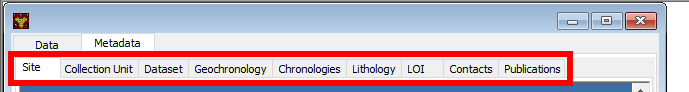
Metadata editing requires information to be entered on the following subtabs:

• Site Tab
• Collection Unit Tab
• Dataset Tab
• Geochronology Tab
• `Chronologies Tab`_
• `Lithology Tab`_
• `LOI Tab`_
• Publications Tab
• Contacts Tab

These tabs are generally arranged in the order of importance as far as a data user might be concerned, but for data entry it often makes sense to start by adding publication & contact information first. This information is used throughout the Tilia file, so it makes sense to enter it first. From here, the rest of the information can be added in any order you wish (and you can navigate to them using the sidebar, or here). For complex records, where you might find yourself writing multiple Tilia files, e.g., when you have multiple collection units or datasets from an individual site, it makes sense to fill in the Publication, Contacts & Site data and save the file as a template. If you have common Chronology information across datasets (for example, a pollen & ostrocode record), then fill in those fields and save the file as a template. This is why it is often helpful to fill in the Metadata first.

Publications Tab

The publications tab is where publication data associated with the record will be stored. This data goes into Neotoma (and may already be stored in Neotoma) as part of the record, but is also stored apart from the collection record.

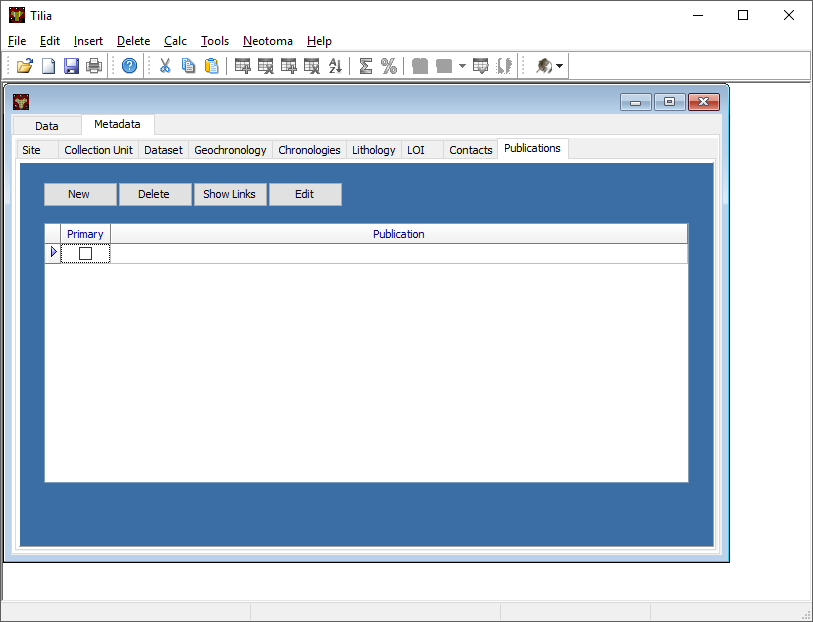
To add a new record click New. Then click on the packrat to check if the publication already exists in the Neotoma database. The easiest way to do this is enter in the author’s last name as a wildcard search. If an appropriate reference shows up, click the reference and then click Use. If not, click Cancel. Choose whether the publication is a journal, book chapter, etc. Then fill in the appropriate fields. Filling in author’s data will also enter data into contacts as well.

Note that if you are adding records via Tilia on a Mac, Tilia freezes when entering new publications. So save often, and perhaps do this step from a PC.

Contacts Tab

Contacts are all individuals related to the record. This includes the individuals who produced & published the record, but also the individuals who assisted in the preparation of chronologies, or in the submission of the data.

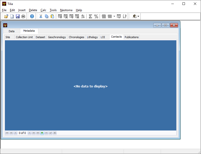
Contacts can (and likely will) be entered as you enter data into the other tabs. You don’t need to enter information in all at once, but you will need to link to individual contacts from a number of tabs (for example the Chronology Tab). If you need to enter a Contact directly, follow the directions below:

First, check to confirm that contact information from the publications tab was entered correctly. Remember, contacts include the authors of the published paper you are entering, yourself (the data enterer), collector(s) and individuals associated with content including the chronology. Contact information for publicaiton authors will have been inserted when entering data in the Publications Tab.

To add a new contact click the green + at the bottom of the window. This should create an empty contact field. Neotoma contains a number of pre-existing contacts, so it’s always best-practice to first search for an individual first. To do this, enter the individual’s family name and then click the Neotoma icon at the end of the field. A new screen will appear. In the search box enter the family name and click the binoculars. If the correct contact is found and all data is up-to-date, click Match and it will be added to the Contacts Tab. If the contact info needs to be updated, click the blue arrow and add any additional information. Then click Update Contact.

If there is not a contact in the database, press OK and then press the blue arrow to transfer the family name from the Tilia Contact to the Neotoma Contact. Fill in any data you can in the Neotoma Contact. Leading initials are the initials of the first and middle names with a period after them. Phone numbers should be entered in the following format: +1-XXX-XXX-XXXX. When all data is entered click Upload Contact.

Site Tab

The Site Tab provides important information about the site and geographic context of the collection you are submitting. Be sure to be as accurate as possible. If you don’t have accurate Latitude/Longitude available it is possible to obtain these values using the Google Maps button, which will provide a map based interface with which to select a location.

Site Name

Use the common name or most popular name used from the publication. Check Neotoma to make sure this name doesn’t already exist.

First Geopolitical Division

Country the site is in.

Second Geopolitical Division

State the site is in.

Third Geopolitical Division

County the site is in.

Administrative Unit

Site is in private, state, federal, etc. land.

Latitude/Longitude

For exact locations, click “Point”. Enter in latitude and longitude. You will have the option to enter in either the decimal, degree or combination of decimal and degree. Enter data as decimals. Click the “Fuzzy” option if you don’t want the exact location of the site made publicly available and choose the radius of the range. If the general locality is unclear, click “Box” and fill in the four coordinate points. Hit OK. To add a bounding box directly from map view, click the google maps icon. A new tab named “Site Locator” will open. Select the “Box” button and N, E, S, W orientations will appear. Select one of the orientation buttons at a time, and click around the pin dropped on the map, to create the perimeter of the bounding box. Doing so will set the north and south latitudes equal and the east and west longitudes equal.

Site Description

Enter in any additional information that describes the general description of the location.

Site Notes

Enter in any additional notes about the locality that may clear up any confusion, such as abbreviations, or changes in the site’s historical naming. Many lakes (for example) have unique identifiers as part of their management by local or regional authorities. These, along with the latitude and longitude can help clarify uncertain naming.

Collection Unit Tab

Handle

Create a unique handle name in all caps. This should be 4-10 letters long.

Collection Unit Type

This is the type of collection you are recording. For mammals, the most common choices will be Excavation, Isolated Specimen, Animal Midden, Surface Float, Midden. For pollen you might select “Core” or “Modern”

Collection Unit Name

If there are multiple collections from the same locality it is important to identify them uniquely. The name should be descriptive of the particular collection (e.g. collection number).

Collection Device/Location in Site

These fields are for collections that use particular field techniques, for example coring devices or other extractive tools.

Collectors

If you have entered these individuals from the Contacts Tab then you will be able to select the individuals from the dropdown menu. If an individual is not selected then navigate to the Contacts Tab to add them. It is best to add all individuals involved in the collection, not just the individuals listed in associated publications.

Date Collected

Record the most accurate date provided. If only the year is known, use January 1st. If only the month and year are known, use the 1st.

Depositional Environment

This will most likely be under terrestrial, so click the arrow next to terrestrial to get more options and search and then click on the appropriate subcategory to get more options.

Substrate

If known use the arrows to get more options and click the appropriate category.

Collection Unit Notes

Any additional information about this specific collection that would be useful to other researchers. (e.g. notes on how the unit was collected, when the unit was collected, etc.)

Slope Angle

Can be obtained in the field. If unknown then leave the field blank.

Slope Aspect

Can be obtained in the field. If unknown then leave the field blank.

Water Depth

Can be obtained in the field. If unknown then leave the field blank.

Dataset Tab

Dataset Type

Vertebrate fauna.

Dataset Name

Unique name to this faunal list (not always necessary to fill out).

Investigators

Who is responsible for the dataset, often but not always the author(s) of the published paper. This information should be available in the Contacts Tab edited earlier.

Publications

Full publication record. Choose the appropriate publications associated with this locality. In general these should have been entered as part of data entry in the Publications Tab. If they have not been, navigate to the Publications Tab and enter this information.

Repository

The museum or institution that houses the collection. If there are repositories that are not currently listed in the drop-down menu contact the Neotoma Paleoecological Database.

Dataset Notes

Any additional notes regarding the dataset, including the locality number for the repository institution (e.g. UCMP V35864).

Data Processors

The person who enters the data into the database.

Spatial Extent

Don’t worry about this box, it’s mainly relevant to aggregate dataset. But if you want to add something, for most cases click Single Stratigraphic. Unclick box if the top sample is not modern surface sample.

Geochronology Tab

The Geochronology tab is central to generating the chronologies for your record. It becomes linked to the Contacts Tab and to the Chronology Tab. The tab contains all geochronological records used for chronology construction. In pracitice most Neotoma records include geochronological data, but this is not always the case.

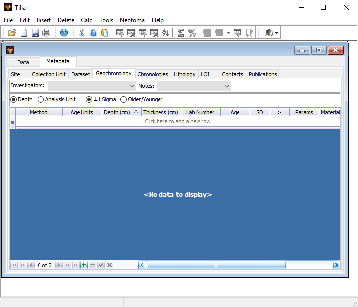
The “Geochronology” metadata tab.

First, at the top add the Investigator name and any notes. Then there is the option to click Depth or Analysis Unit. If the site has individually dated layers with depth and thickness data, then choose Depth. If the site is an assemblage, choose Analysis Unit. Since you have added this information into the Data tab, it should be automatically linked (at least the Analysis Unit info). Click the green + button at the bottom to add a new record, or just start typing in row 1.

Method

Use the drop down menu to choose the appropriate dating method. This will be Carbon-14 in the majority of cases.

Age Units

Use the drop down menu.

Depth

Depth of the unit that is dated. Optional depth of the Analysis Unit in cm. Depths will typically be designated for Analysis Units from cores and for Analysis Units excavated in arbitrary (e.g. 10 cm) levels.

Thickness

The thickness of the dated unit.

Analysis Unit

This will most likely be an assemblage.

Lab Number

The lab number of that sample.

Age

The raw age of the sample.

SD

The standard deviation of the raw age.

Params

Click on the empty cell and a drop down box will appear. Click in the cell to the right of Methods and choose a dating method (e.g. accelerator mass spectrometry).

Material Dated

What kind of material was dated (free-form text entry)

Publication

Choose the publication from the drop down menu. (This should appear after entering the contact information.)

Click the green Check mark to post your edits once you’re done. The row you’ve just edited will get pushed down below the header. You’re not done quite yet. There’s still more information to add.

Once the record gets added to the Geochronology for the collection, you can add more information to the record. To do this, click the “+” tab at the front of the row. A sub-row will appear.

ID

This will fill in automatically. Leave it blank.

Taxon

The taxon name for organic elements.

Element

Use the pull down menu to select the element that was dated. This is defined in part by the `Lookup Table`_ you’ve decided to use.

Fraction

Use the pull down menu to select how the element/specimen was prepped for dating. There are a pre-defined set of terms for use, including “Unknown”, but you can also add your own terms if the available terms aren’t appropriate.

Cal Age Older/Younger

These are the calibrated dates for the samples. You have two options here:

1. Enter the calibrated ages by hand if they are provided in the paper (or you’re handy with an Intcal table)
2. Calibrate ages using Tilia. To do this, click Tools in the menu bar and then Calibrate. In the new menu put in the age of the sample and the standard deviation and press Go. This will automatically provide an older and younger calibrated age.

Cal Curve

This is the calibration curve used to generate the calibrated dates. If you used Tilia to calculate the date this will be Intcal13. If you used something else to calibrate the age (or if it was provided from a publication), choose the appropriate calibration curve from the drop down menu.

Cal Program

Choose the calibration program that was used to generate the calibrated date.

Click the green check at the bottom to post the changes.

If you have more than one dated sample for this geochronology element, click the green + at the bottom of the page and add a second record. Continue process until all samples are recorded.

Chronology Tab

The Chronology tab is separate from the Geochronology Tab. Geochronology stores information about dated samples based on radiometric or similar geochronological methods, while Chronology stores the key metadata for a given age model. As part of this metadata, Chronology stores all of the age controls used as constraints for an age model. This list can include some, none, or all of the radiometric dates stored in Geochronology, and also can include non-radiometric age controls (such as a core-top in a sediment core, a biostratigraphic event of known age, etc). This design may seem a little odd at first, but it serves the very useful function of allowing a lot of user flexibility in putting together age models.

To get started, open the “Chronologies” tab and click within the white bar containing the text “Click here to add a new row”.

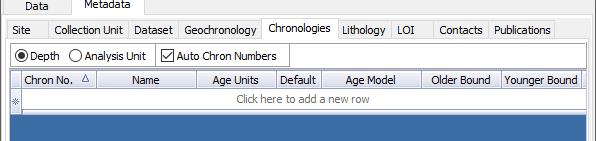
You will see that the solid bar becomes divided into cells when you click. For each cell fill in the appropriate information:

Name

A name for the chronology. Give the Chronology a descriptive name (it’s a good rule of thumb not to just use “linear” or “Bacon” since you might make multiple models using the same method).

Age Units

The chronology age units. This is a drop-down selection & does not permit multiple selections.

Default

If you have only one model click the “Default” box. Otherwise, if you have multiple models, decide which model will be the default. This decision is important. Once the data goes up to Neotoma the default model will be the one used in searches and to display the data. Only one record can be the Default.

Age Model

The “Age Model” cell is where you will describe the model used, for example “clam - linear”.

Older/Younger Bound

The oldest & youngest ages of the model (used for searching). Be careful here. In a bootstrapped or Bayesian model it is possible to get estimates that are well beyond the range of acceptable values, particularly if you extrapolate below dated material. Generally, the protocol is that the Older Bound is rounded up to the nearest 10 years and the Younger Bound is rounded down, e.g. if the sample age bounds are -44 to 10773, the Older Bound would be 10780 and the Younger Bound would be -50.

Preparers

These are obtained from the Contacts Tab list. If the Preparer is not already in that list then it is best to fill them in and then continue with the chronology tab. (NOTE: read below first)

Date Prepared

When did you generate the age model? This drop down menu provides a calendar, which is a nice touch.

Notes

For more complex models including Bacon it is standard protocol to copy the settings into this field. Otherwise this is a “free-form” cell.

Once the fields have been filled, click the tiny “+” sign at the bottom of the window.

This adds the entered data into the Chronology tray, allowing us to associate more data with the record. Now we need to associate Geochronological data with the Chronology we’ve just created. To begin this, we need to add the data from the Geochronology Tab to our chronology. To do this we expand the Chronology we just created. We do this by clicking the “+” sign at the beginning of the row (in the figure below).

Once you’ve clicked the “+” button you’ll see a new spreadsheet. By clicking into the spreadsheet you will cause new buttons to appear under the Metadata Tabs. The buttons say “Link”, “Import” and “Export”. If you’ve already entered the Geochronological data into the metadata table, all you need to do is click “Import”. A new window will appear (below). Select the appropriate values.

In general it makes sense to use the defaults unless there is a very good reason to do so.

At this point you can enter any extra (non-geochron) dates that you may have used in generating your age model. The idea here is that this table will reflect the input data used to generate your age model. For example, to add a “Core Top” date enter data in the top row, and then select Age Basis > “Stratigraphic” > Core Top. You’ll see a number of options under these fields.

In cases where you are being proactive (congratulations!) and entering your data before you’ve built your age model, you may have enough information to construct a proper chronology, which allows you to estimate the ages of undated depths. If you want to use Bacon or Clam to build your chronology then you can click the Export button at the top of the Chronologies worksheet.

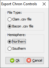
This will save the appropriate csv file for Bacon or Clam (in this case, make sure you have dates entered in the Data Tab). You can then build your age model using R and import the age model back into your record (discussed in the Data Tab section).

If you do use Bacon or Clam to generate your interpolated chronology then remember to copy your settings file into the Notes field. This will allow people to replicate your results.

Annotating the Data

In some cases, analysts may want to add extra data that describes the Analysis Units. The most typical type of data to add is information about the ages associated with each depth (see below), but other forms of metadata can be added such as analysis unit thicknesses or sample analyst.

To add, e.g., analysis unit thickness, add a blank row UNDER the Analysis Unit name (ie, in row 3). To do this, hover your mouse over cell A3, then right click in the top left cell of that row, and select Metadata → Analysis Unit → Thickness. You will see that a new row has been added, with an associated code and name for the variable. You can then proceed to enter values for analysis unit thickness starting at Column H.

Adding the Chronology

Once the age model information is added to the Chronology table, navigate back to the Data tab. Here we can import the dates for the model. There are two options. If you want Tilia to build the model for you you can select Tools > Chronology. If you’ve built the model yourself using Bacon or Clam then you can import the output file directly using Tools > Import Chronology > Bacon/Clam. If you have a record for which the age model is entirely made up of directly dated objects (or absolutely dated records) where the Chronology tab sheet is equivalent to the actual depths/records in the Data sheet then it is possible to directly import the Chronology Tab Sheet using Tools > Import Chronology > Chronologies Tabsheet.

To add the chronology from Bacon or Clam that you have already created, Go to Tools > Import Chronology > Bacon/Clam. Your Chronologies have numbers associated with them in the Chronologies Tab. Make sure you’re using the right Chronology number. Bacon and Clam have different options, but you should choose the right file and the age values that make the most sense to you.

Once you click OK, navigate to the appropriate file and click okay. The chronology will be added to the Data tab.

Common Issues: I’ve imported my chronology, but the ages don’t appear in the Data spreadsheet!

System Message: ERROR/3 (/home/docs/checkouts/readthedocs.org/user_builds/tilia-manual/checkouts/latest/docs/edit_data.rst, line 325)

Unexpected indentation.

The usual cause of this error is a misalignment between the depths of samples in Tilia’s Data spreadsheet and the depths listed in _ages.txt file outputted by Bacon or Clam. Tilia looks for exact matches, so e.g. if the depths of samples in the Tilia file are 0.5 10.5 20.5… and the depths in the …_ages.txt file are 1 2 3 4 5 6 …. then there are no exact matches and no ages will be imported into the Tilia file. There are a couple of possible workarounds (e.g. hand-editing the _ages.txt file) but usually the best solution is to rerun Bacon or Clam with a _depths.txt input file that contains all the depths listed in the Data spreadsheet. Bacon or Clam will then output an _ages.txt file that should import cleanly into Tilia, suing the steps above.